Perfect Competition

Perfect competition refers to a market structure where competition among the sellers and buyers prevails in its most perfect form. In a perfectly competitive market, a single market price prevails for the commodity, which is determined by the forces of total demand and total supply in the market.

The following features characterize a perfectly competitive market:

a) A large number of buyers and sellers: The number of buyers and sellers is large and the share of each one of them in the market is so small that none has any influence on the market price.

b) Homogeneous product: The product of each seller is totally undifferentiated from those of the others.

c) Free entry and exit: Any buyer and seller is free to enter or leave the market of the commodity.

d) Perfect knowledge: All buyers and sellers have perfect knowledge about the market for the commodity.

e) Indifference: No buyer has a preference to buy from a particular seller and no seller to sell to a particular buyer.

f) Non-existence of transport costs: Perfectly competitive market also assumes the non-existence of transport costs.

g) Perfect mobility of factors of production: Factors of production must be in a position to move freely into or out of industry and from one firm to the other.

AR (Average revenue) curve and MR (Marginal Revenue) curve under perfect competition becomes equal to D (Demand) curve and it would be a horizontal line or parallel to the X-axis. The curve simply implies that a firm under perfect competition can sell as much quantity as it likes at the given price determined by the industry i.e. a perfectly elastic demand curve.

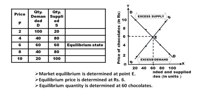
Price is determined by the market forces, that is, demand and supply for a given product or service. As discussed above, firms have no control over the prices they charge for their products. The ultimate price that determines the quantity demanded is equal to the quantity supplied. This price is also called equilibrium price, as it balances the forces of demand and supply. The figure shows how the price is determined. DD is the demand curve and SS is the supply curve. Rs. 6 is the price at which DD and SS intersect each other. At Rs. 6, 60 units are supplied and demanded.

If the price increases to Rs. 8, supply will also increase and hence the price is likely to fall down.

If the price decreases to Rs. 4, supply will decrease and hence the price is likely to go up.

In this market, the price is determined by supply and demand forces. Marshal, who propounded the theory, says that the price is determined by the equilibrium between demand and supply.

The pricing of commodity under perfect competition can be determined in three periods of time:

a) Very short period (Market Period): Market period is too short a period to increase the supply. The market period is so short that supply of the commodity is limited to existing stock. During the market period, say a single day, the supply of a commodity is perfectly inelastic.

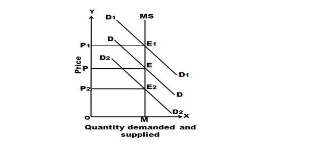
In this figure quantity is represented along X-axis and price is represented along Y-axis. MS is the very short period supply curve. DD is demand curve. It intersects supply curve at E. The price is OP. The quantity is OM. D1 D1 represents increased demand. This curve cuts the supply curve at E1. Even at the new equilibrium, supply is OM only. But price increases to OP1. So, when demand increases, the price will increase but not the supply. If demand decreases new demand curve will be D2 D2. This curve cuts the supply curve at E2. Even at this new equilibrium, the supply is OM only. But price falls to OP2. Hence in very short period, given the supply, it is the change in demand that influences price. The price determined in a very short period is called Market Price.

b) Short Period: Short period is not too long a period to install new capital equipment. It is also not a sufficient period to permit the new firms to enter the industry to increase the supply of the commodity in the market. Hence the firm can increase the supply of a commodity in the short period only by making intensive use of the given plants and equipment and increasing the units of variable factors. As a result of this, the short period supply of a commodity will be relatively less elastic.

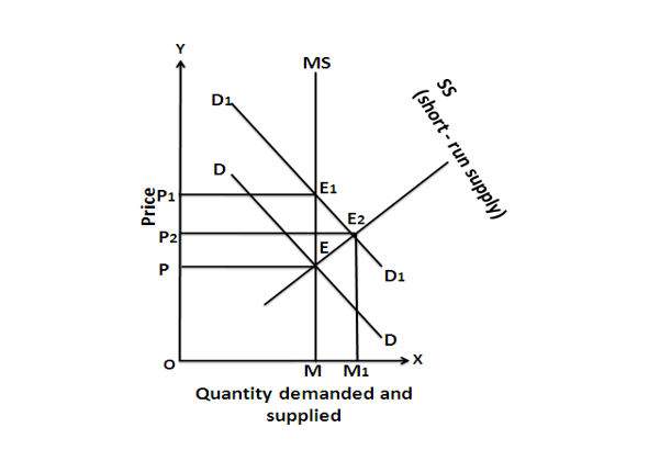
In the diagram MS is the market period supply curve. DD is the initial demand curve. It intersects MS curve at E. The price is OP and output OM. Suppose demand increases, the demand curve shifts upwards and becomes D1D1. In the very short period, supply remains fixed on OM. The new demand curve D1D1 intersects MS at E1. The price will rise to OP1. This is what happened in the very short period. As the price rises from OP to OP1, firms expand output. As firms can vary some factors but not all, the law of variable proportions operates. This results in new short-run supply curve SS. It intersects D1 D1 curve at E2. The price will fall from OP1 to OP2.

c) Long Period: In the long run, the firm’s output (supply) can be changed by both the variable factors and fixed factors i.e. all factors become variable. There is enough time for new firms to enter the industry. Further, if the demand is increased, the supply can be increased or decreased according to the demand. For long-run equilibrium, long-run marginal cost (LMC) is equal to MR and LMC curve cuts the MR curve from below. In case of long-run equilibrium, all the firms will earn only normal profits.

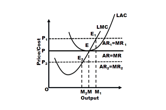
Take the case when the firm earns super-normal profit: Then the existing firm will increase their production and new firms will enter the industry. Consequently, the total supply will increase and price will fall down and further result in normal profit for the firm. On the contrary, if the firm is incurring losses, then some firms will leave the industry which will reduce the total supply. And due to decrease in supply, price will rise and once again firms will begin to earn normal profit. Firm equilibrium is at the minimum point of its LAC and at this point the firm will get normal profits. If AR (price) rises to OP1, then firm’s LMC cuts its MR1 at E1 and the firm gets super-normal profit but again comes to OP yielding normal profits as stated before. And at price OP2, firm incurs losses but again rises to level OP to maintain the equilibrium at normal profit.

Firm’s equilibrium: MC=MR=AR=min LAC