Cost-Output Relationship
The cost-output relationship plays an important role in determining the optimum level of production. Knowledge of the cost-output relationship helps the manager in cost control, profit prediction, pricing, promotion, etc. Output is an important factor that influences cost. Considering the period, the cost function can be classified as:
Under the short-run cost-output relation, costs are classified into fixed costs and variable costs. Labour is the variable factor while capital is the fixed factor. Total fixed cost remains constant while variable cost changes with the variation in units of labour. The fixed costs may be ascertained in terms of total fixed cost and average fixed cost per unit. The relationship of costs in the short run can be summarized as follows:
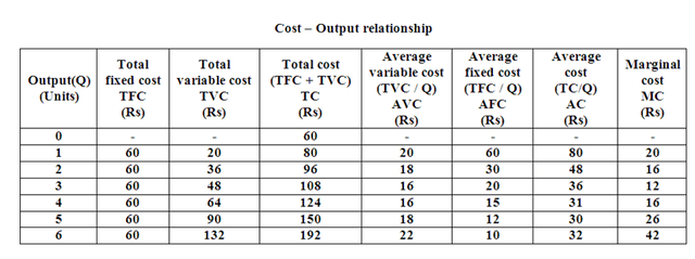
– Total fixed costs remain fixed irrespective of the increase or decrease in production activity.
– Average fixed cost per unit declines as the volume of production increases due to spreading fixed costs over more units.
– Total variable cost increases proportionately with production.
– Total cost increases with the volume of production.
– Average total cost initially decreases up to a certain level of production, then rises, forming a U-shaped curve.
– Marginal cost reflects the change in total cost due to one unit change in output.
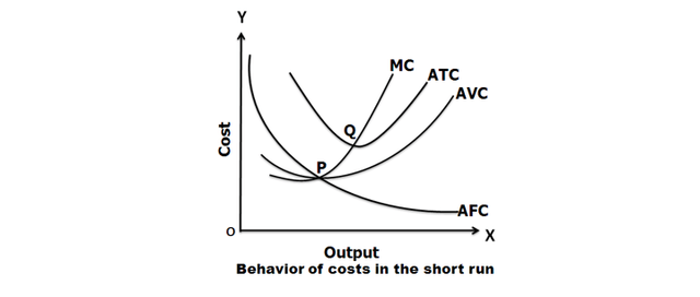
The short-run cost-output relationship can be illustrated graphically as follows:
– The Average Fixed Cost (AFC) curve slopes downwards continuously as production increases.
– The Average Variable Cost (AVC) curve is U-shaped, initially falling and then rising due to the law of diminishing returns.
– The Average Total Cost (ATC) curve initially declines with AVC but rises after a certain production level.
– Marginal Cost (MC) initially decreases with output but later increases steeply.
Long run refers to that period of time over which all factors are variable. It has no fixed cost. Over a long period, the size of the plant can be changed, unwanted buildings can be sold, staff can be increased or reduced. The long run enables the firms to expand and scale their operation by bringing or purchasing larger quantities of all the inputs. Thus, in the long run, all factors become variable.
In the long run, a firm has a number of alternatives regarding the scale of operations. For each scale of production or plant size, the firm has appropriate short-run average cost curves. The short-run average cost (SAC) curve applies to only one plant whereas the long-run average cost (LAC) curve takes into consideration many plants.
If we assume that there are many plant sizes, each suitable for a certain level of output, we will get many SAC curves intersecting each other. As the number of plant sizes increases, the points of intersection of SAC curves will come closer. And, if we assume that there are a large number (say, an infinite number) of plant sizes, the intersection points will be so near to each other that we get almost a continuous curve. This continuous curve is known as the Long-run Average Cost (LAC) curve or the Envelope curve (as it envelopes the family of short-run Average Cost Curves).
The long-run cost-output relationship is shown graphically with the help of the LAC curve.
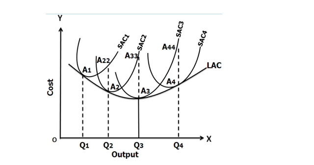
The above figure shows how the LAC curve envelopes several short-run average cost (SAC) curves. Suppose, the firm is producing an output of OQ1 units on a plant of SAC1, if it wants to produce OQ2 units of output, either it can operate on SAC1 by over-utilizing the SAC1 plant or by acquiring a bigger size plant SAC2 and operating on it. It will be less costly to operate on SAC2. If it wants to produce OQ3 units of output, it can operate on the bigger size plant SAC3 at least cost. Q3A3 is the least cost at the output OQ3 and the firm attains optimum output in the long run at OQ3 level of output. If it operates on SAC2 to produce OQ3 units of output, the cost will be prohibitively high being Q3A3. It is to be noted that there is only one short-run average cost curve SAC3 which is tangential to the long-run average cost curve at its minimum point. All other SAC curves are tangential to the LAC curves at higher than their minimum average cost points.